Monte Carlo Options Pricing - GPU Accelerated Simulation
Last reviewed: by Options Analysis Suite Research.
What Is Monte Carlo Pricing?
Monte Carlo pricing values an option by simulating thousands or millions of price paths
under a chosen model's risk-neutral dynamics, computing the option's payoff on each path,
discounting to present value, and averaging. The strength of Monte Carlo is generality:
any payoff function and any path-dependent feature can be priced as long as you can simulate
the underlying. The cost is computational expense and statistical noise that converges
only as 1/√N in the number of paths.
Monte Carlo is the workhorse for exotic options (barriers, Asians, lookbacks), for any multi-asset payoff, and for risk-neutral probability distributions where you want the full histogram of outcomes rather than a single price. It's also the tool of choice when your model lacks a closed-form characteristic function: Local Volatility, Variance Gamma with stochastic variance, jump-diffusion-with-jump-clustering, and other research-grade dynamics fit here.
The Algorithm
- Choose a model (Black-Scholes, Heston, Local Vol, Jump Diffusion) and discretize the SDE: typically Euler, Milstein, or QE for Heston.
- Generate N independent path realizations using normally-distributed shocks at each time step. Antithetic variates and quasi-random sequences (Sobol, Halton) reduce variance vs naive pseudo-random.
- For each path, compute the payoff at expiration (or path-dependent payoff for exotics).
- Discount each payoff to present value using the risk-free rate.
- Average across all paths; this is the Monte Carlo price estimate. The standard error of the estimate is
σ_payoff / √N.
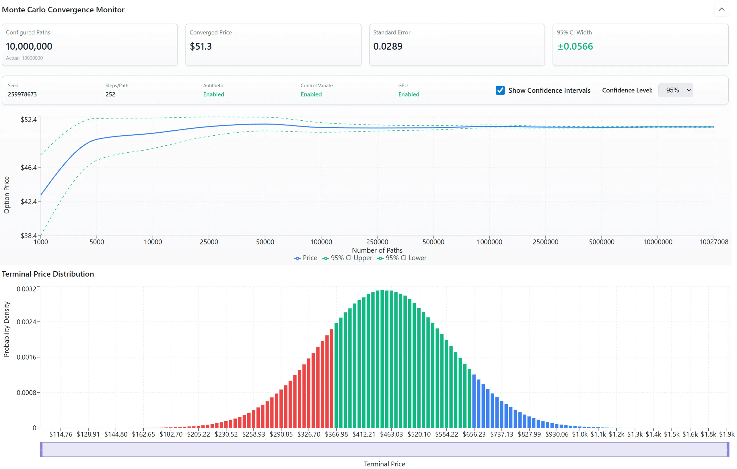
How Do You Improve Monte Carlo Convergence?
Naive Monte Carlo with N = 10,000 paths gives you roughly a 1% standard error on a vanilla ATM option, usable for sanity checks but not for tight calibration. Variance reduction techniques tighten this materially:
- Antithetic variates: pair every path with its sign-flipped twin to cancel symmetric noise. Roughly halves variance on most payoffs.
- Control variates: pair the exotic with a vanilla that has a closed-form Black-Scholes price; subtract the simulated vanilla and add back the closed-form. Works well when the exotic and the control are highly correlated.
- Quasi-random (low-discrepancy) sequences: Sobol or Halton sequences fill space more uniformly than pseudo-random, accelerating convergence to
(log N)d/Nfrom1/√N. - GPU acceleration: Monte Carlo is embarrassingly parallel; the platform's GPU pricer runs millions of paths in seconds.
When Should You Use Monte Carlo?
- Exotic options with path-dependent payoffs (Asian, barrier, lookback, double-barrier).
- Multi-asset options (basket, rainbow, best-of, worst-of) where the joint distribution matters.
- Risk-neutral probability distributions: the full histogram of
S_T, not just a single mean. - Any model where the characteristic function is unknown or numerically unstable.
When Should You Not Use Monte Carlo?
- Vanilla European options where Black-Scholes or Heston-FFT gives you the same answer in microseconds with zero noise.
- American options: early exercise requires Longstaff-Schwartz regression, which is slower and less stable than the binomial tree or PDE approach for most retail use cases.
- When you need precise Greeks: Monte Carlo Greeks via finite differences are noisy; pathwise or likelihood-ratio Greeks are better but more complex to implement.
Discretization and Numerical Stability
The choice of discretization scheme matters significantly for Monte Carlo accuracy.
Euler-Maruyama is the simplest scheme: St+Δt = St · exp((μ − σ²/2)·Δt + σ·√Δt·Z)
where Z is a standard normal. It converges to the correct distribution as Δt → 0 but
introduces discretization bias on coarser grids. Milstein adds a second-order term that
reduces the bias for stochastic-volatility models like Heston. For Heston specifically,
the Quadratic Exponential (QE) scheme by Andersen handles the variance process near zero
cleanly. Naive Euler discretization of Heston can produce negative variances, which
breaks the model. QE is the production-grade method for Heston Monte Carlo and is what
production pricers use.
How Do You Improve Monte Carlo Convergence?
Naive Monte Carlo with N = 10,000 paths gives roughly a 1% standard error on a vanilla ATM option, usable for sanity checks but not for tight calibration. Variance reduction techniques tighten this materially:
- Antithetic variates: pair every path with its sign-flipped twin to cancel symmetric noise. Roughly halves variance on most payoffs at zero additional simulation cost beyond the matched generation.
- Control variates: pair the exotic with a vanilla that has a closed-form Black-Scholes price; subtract the simulated vanilla and add back the closed-form. Works well when the exotic and the control are highly correlated, which is typical for vanilla-similar exotics.
- Quasi-random (low-discrepancy) sequences: Sobol or Halton sequences fill the path space more uniformly than pseudo-random, accelerating convergence to
(log N)d/Nfrom1/√N. The improvement is dimension-dependent and weakens for very high-dimensional payoffs. - Importance sampling: shift the simulation measure toward regions that contribute most to the payoff (e.g., toward the strike for OTM options). Reduces variance dramatically when applicable but requires payoff-specific tuning.
- GPU acceleration: Monte Carlo is embarrassingly parallel; the platform's GPU pricer runs millions of paths in seconds rather than minutes.
When Should You Use Monte Carlo?
- Exotic options with path-dependent payoffs (Asian average, barrier knock-in/out, lookback, double-barrier, cliquet). The path-by-path simulation handles arbitrary payoff specifications.
- Multi-asset options (basket, rainbow, best-of, worst-of) where the joint distribution matters and pricing requires correlated random variates across the asset set.
- Risk-neutral probability distributions: the full histogram of
ST, not just a single mean. Useful for probability-of-profit calculations on multi-leg strategies. - Any model where the characteristic function is unknown or numerically unstable. Custom research models often only have a Monte Carlo evaluation path.
- Validation of analytical pricers: Monte Carlo with sufficient paths converges to the analytical answer for vanilla options, providing a cross-check on closed-form implementations.
When Should You Not Use Monte Carlo?
- Vanilla European options where Black-Scholes or Heston-FFT gives the same answer in microseconds with zero noise. Monte Carlo overhead is not justified for closed-form-friendly cases.
- American options: early exercise requires Longstaff-Schwartz regression to estimate the continuation value, which is slower and less stable than the binomial tree or PDE approach for most retail use cases.
- When you need precise Greeks: Monte Carlo Greeks via finite differences are noisy; pathwise or likelihood-ratio Greeks are better but more complex to implement and don't apply to all payoffs.
- For options where only the price is needed and an analytical or numerical-PDE method is available, choose the lower-noise method.
How OAS Uses Monte Carlo
The platform offers GPU-accelerated Monte Carlo for any of the supported models, with
configurable path counts, antithetic variates, and Sobol sequencing. Risk-neutral probability
distributions on per-ticker pages use Monte Carlo to produce the full payoff histogram, not
just a single expected value. The Python SDK exposes a full mode that returns
the path matrix for downstream research; the standard price mode returns the
converged estimate plus its standard error. For Heston, the platform uses the QE
discretization scheme to preserve variance non-negativity, which keeps the simulation
statistically consistent with the model under realistic parameter regimes.
Run Monte Carlo in the pricing calculator
Related Concepts
Risk-Neutral Probability · Heston (via MC) · Jump Diffusion (via MC) · Variance Gamma (via MC) · Local Volatility (via MC) · Black-Scholes · PDE Methods · FFT Pricing · Greeks Reference · Risk-Neutral Density · Tail Risk · Model Landscape
Try this model in the pricing calculator
This section is part of the Options Analysis Suite Documentation. Browse the full model index or compare alternatives in the pricing calculator.