FFT Options Pricing - Fast Fourier Transform
Last reviewed: by Options Analysis Suite Research.
What Is FFT Pricing?
FFT (Fast Fourier Transform) pricing is a numerical method for pricing options whenever
the underlying model has a known characteristic function. The technique, popularized by
Carr and Madan (1999), evaluates a Fourier-domain integral over the characteristic
function and uses the FFT to compute prices for a whole grid of strikes simultaneously
in O(N log N) time. For models like Heston, Variance Gamma, and CGMY where
the characteristic function is closed-form but no analytic price exists, FFT is the
fastest practical pricer.
FFT is what makes calibration tractable for stochastic-volatility and Lévy models. A calibration loop needs to price hundreds of options per iteration; without FFT, the Heston calibration that the platform runs in seconds would take minutes per fit.
How It Works
The Carr-Madan formulation transforms the call price into a damped Fourier integral:
multiply the call price by e^(αk) for some damping factor α > 0,
and the resulting function has an integrable Fourier transform expressible directly via
the characteristic function of ln(S_T). Evaluating this integral on a
discrete grid via the FFT gives prices at log-strikes spaced 2π/(N·η) apart
in one shot.
What Is FFT Good For?
- Vanilla European options under Heston, Bates, Variance Gamma, CGMY, and other Lévy / stochastic-volatility models with closed-form characteristic functions.
- Calibration loops where pricing the entire surface fast matters more than pricing a single option.
- Moment-based diagnostics: risk-neutral skewness, kurtosis, and other distribution moments are direct outputs of the characteristic function.
What Isn't FFT Good For?
- Path-dependent exotics: FFT prices European payoffs only.
- American options: early exercise breaks the Fourier-transform approach; PDE or binomial trees are needed.
- Models without a closed-form characteristic function: Local Volatility and many regime-switching models don't fit.
- Pricing single options with high precision: the FFT grid has discretization error at strikes far from the grid centers; Fourier-COS or numerical integration is sometimes more accurate per-strike.
The Damping Factor and Numerical Considerations
The damping factor α in the Carr-Madan formulation is a tuning parameter that affects numerical stability. Too small and the integrand decays slowly, requiring many grid points to capture the integral accurately. Too large and the integrand becomes oscillatory at the grid edges, introducing aliasing errors. Production implementations use α between 0.5 and 2.0 depending on the model and the price range being computed, often with adaptive selection based on the moneyness and tenor of the target options. The grid spacing η and grid size N also matter: smaller η produces tighter strike-grid resolution but at higher cost, and N must be a power of 2 for the FFT to work efficiently (N = 2¹² or 2¹⁴ are typical). Carr-Madan grid effects are well-understood; the Fourier-COS method by Fang and Oosterlee provides an alternative formulation that often converges faster and avoids some of the grid-spacing tradeoffs.
Calibration Loops and FFT
FFT pricing is what makes calibration of stochastic-vol and Lévy models tractable. A typical calibration loop reprices a few hundred options against listed market prices at each iteration, and the optimizer typically converges in 20-100 iterations, meaning tens of thousands of option prices are computed per fit. With closed-form pricing (Black-Scholes), this is trivially fast. Without FFT, Heston calibration would need Monte Carlo simulation per option, which is orders of magnitude slower and produces noisy prices that destabilize the optimizer. The closed-form characteristic function plus FFT pricing is what makes Heston, Variance Gamma, Bates, and similar models practical to calibrate nightly across thousands of tickers.
What Is FFT Good For?
- Vanilla European options under Heston, Bates, Variance Gamma, CGMY, and other Lévy / stochastic-volatility models with closed-form characteristic functions.
- Calibration loops where pricing the entire surface fast matters more than pricing a single option with maximum precision.
- Moment-based diagnostics: risk-neutral skewness, kurtosis, and other distribution moments are direct outputs of the characteristic function and don't require additional simulation.
- Producing IV surfaces for any model with a closed-form characteristic function: the FFT grid produces prices at all strikes simultaneously, which after Black-Scholes inversion gives a smooth IV surface.
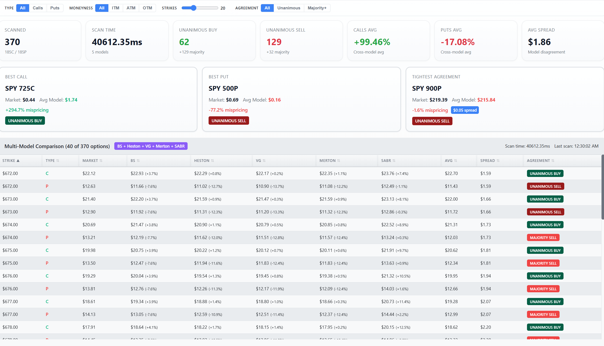
- Cross-model comparison views where every model in the lineup needs to be priced on the same strike grid in the same compute window.
What Isn't FFT Good For?
- Path-dependent exotics: FFT prices European payoffs only. Asians, barriers, and lookbacks need Monte Carlo or PDE methods.
- American options: early exercise breaks the Fourier-transform approach because the optimal stopping time depends on the path, not just the terminal distribution. PDE or binomial trees are needed.
- Models without a closed-form characteristic function: Local Volatility and many regime-switching models don't fit the FFT framework directly.
- Pricing single options with high precision: the FFT grid has discretization error at strikes far from the grid centers; Fourier-COS or numerical integration is sometimes more accurate per-strike for high-precision applications.
How OAS Uses FFT
FFT is the pricing engine behind the platform's Heston, Variance Gamma, Bates, and CGMY surfaces. Calibration fits the characteristic function's parameters by minimizing the error between FFT-priced and listed market prices, typically with Levenberg-Marquardt or a similar gradient-based optimizer working in Black-Scholes IV space rather than dollar prices. The same machinery powers the model-divergence views, which require pricing every option under multiple models in real time. For research, the Python SDK exposes the raw characteristic-function evaluations so users can compose their own FFT-based pricers or moment computations beyond the standard call/put outputs.
Use FFT pricing in the calculator
Related Concepts
Heston (via FFT) · Variance Gamma (via FFT) · Jump Diffusion · Black-Scholes · Monte Carlo · PDE Methods · Calibration · Risk-Neutral Density · Model Divergence · Model Landscape
Try this model in the pricing calculator
This section is part of the Options Analysis Suite Documentation. Browse the full model index or compare alternatives in the pricing calculator.